Viewing Dataframes
After you successfully request a dataset from the USGS, Hydrofunctions will process the data into a huge table and make it available to you in several formats.
If you are working with Python and timeseries data, then you should already know about Pandas and Numpy, the numerical systems Hydrofunctions is built upon. These two data analysis packages are involved in almost all scientific data analysis, and are the starting point for hundreds of projects.
Use the following dataset for the examples below:
[1]:
import hydrofunctions as hf
%matplotlib inline
data = hf.NWIS(['01650800', '01589330'], 'iv', start_date='2019-05-01', end_date='2019-06-01', file='view-example.parquet')
Reading data from view-example.parquet
This dataset has the following properties:
[2]:
data
[2]:
USGS:01589330: DEAD RUN AT FRANKLINTOWN, MD
    00060: <5 * Minutes>  Discharge, cubic feet per second
    00065: <5 * Minutes>  Gage height, feet
USGS:01650800: SLIGO CREEK NEAR TAKOMA PARK, MD
    00010: <5 * Minutes>  Temperature, water, degrees Celsius
    00060: <5 * Minutes>  Discharge, cubic feet per second
    00065: <5 * Minutes>  Gage height, feet
    00095: <5 * Minutes>  Specific conductance, water, unfiltered, microsiemens per centimeter at 25 degrees Celsius
    00300: <5 * Minutes>  Dissolved oxygen, water, unfiltered, milligrams per liter
    00400: <5 * Minutes>  pH, water, unfiltered, field, standard units
    63680: <5 * Minutes>  Turbidity, water, unfiltered, monochrome near infra-red LED light, 780-900 nm, detection angle 90 +-2.5 degrees, formazin nephelometric units (FNU)
Start: 2019-05-01 04:00:00+00:00
End:   2019-06-02 03:55:00+00:00
It includes two sites, with seven different types of data being collected at one site, and two at the other.
View the entire table
Let’s start by viewing all of the columns in the first five rows of our table. To view all of our data as a dataframe, we use the .df() method of NWIS. The .head() method limits display of our table to just the first five rows:
[3]:
data.df().head()
[3]:
| USGS:01589330:00060:00000_qualifiers | USGS:01589330:00060:00000 | USGS:01589330:00065:00000_qualifiers | USGS:01589330:00065:00000 | USGS:01650800:00010:00000_qualifiers | USGS:01650800:00010:00000 | USGS:01650800:00060:00000_qualifiers | USGS:01650800:00060:00000 | USGS:01650800:00065:00000_qualifiers | USGS:01650800:00065:00000 | USGS:01650800:00095:00000_qualifiers | USGS:01650800:00095:00000 | USGS:01650800:00300:00000_qualifiers | USGS:01650800:00300:00000 | USGS:01650800:00400:00000_qualifiers | USGS:01650800:00400:00000 | USGS:01650800:63680:00000_qualifiers | USGS:01650800:63680:00000 | |
|---|---|---|---|---|---|---|---|---|---|---|---|---|---|---|---|---|---|---|
| datetimeUTC | ||||||||||||||||||
| 2019-05-01 04:00:00+00:00 | P | 1.99 | P | 0.51 | P | 17.9 | P | 8.98 | P | 1.06 | P | 574.0 | P | 7.6 | P | 7.3 | P | 10.3 |
| 2019-05-01 04:05:00+00:00 | P | 1.99 | P | 0.51 | P | 17.8 | P | 8.65 | P | 1.05 | P | 580.0 | P | 7.6 | P | 7.3 | P | 9.7 |
| 2019-05-01 04:10:00+00:00 | P | 1.99 | P | 0.51 | P | 17.8 | P | 8.65 | P | 1.05 | P | 587.0 | P | 7.6 | P | 7.3 | P | 9.1 |
| 2019-05-01 04:15:00+00:00 | P | 1.99 | P | 0.51 | P | 17.8 | P | 8.34 | P | 1.04 | P | 592.0 | P | 7.6 | P | 7.3 | P | 8.2 |
| 2019-05-01 04:20:00+00:00 | P | 1.85 | P | 0.50 | P | 17.7 | P | 8.03 | P | 1.03 | P | 597.0 | P | 7.6 | P | 7.3 | P | 7.9 |
This is equivalent to data.df('all').head()
We now have nine different columns containing data. Each column has a twin ‘qualifiers’ column, which contains metadata flags.
You can list the columns separately by viewing the columns attribute of the dataframe:
[4]:
data.df().columns
[4]:
Index(['USGS:01589330:00060:00000_qualifiers', 'USGS:01589330:00060:00000',
       'USGS:01589330:00065:00000_qualifiers', 'USGS:01589330:00065:00000',
       'USGS:01650800:00010:00000_qualifiers', 'USGS:01650800:00010:00000',
       'USGS:01650800:00060:00000_qualifiers', 'USGS:01650800:00060:00000',
       'USGS:01650800:00065:00000_qualifiers', 'USGS:01650800:00065:00000',
       'USGS:01650800:00095:00000_qualifiers', 'USGS:01650800:00095:00000',
       'USGS:01650800:00300:00000_qualifiers', 'USGS:01650800:00300:00000',
       'USGS:01650800:00400:00000_qualifiers', 'USGS:01650800:00400:00000',
       'USGS:01650800:63680:00000_qualifiers', 'USGS:01650800:63680:00000'],
      dtype='object')
Viewing only the data columns
To omit the ‘qualifier’ columns from our dataframe, only ask for the nine ‘data’ columns:
[5]:
data.df('data').head()
[5]:
| USGS:01589330:00060:00000 | USGS:01589330:00065:00000 | USGS:01650800:00010:00000 | USGS:01650800:00060:00000 | USGS:01650800:00065:00000 | USGS:01650800:00095:00000 | USGS:01650800:00300:00000 | USGS:01650800:00400:00000 | USGS:01650800:63680:00000 | |
|---|---|---|---|---|---|---|---|---|---|
| datetimeUTC | |||||||||
| 2019-05-01 04:00:00+00:00 | 1.99 | 0.51 | 17.9 | 8.98 | 1.06 | 574.0 | 7.6 | 7.3 | 10.3 |
| 2019-05-01 04:05:00+00:00 | 1.99 | 0.51 | 17.8 | 8.65 | 1.05 | 580.0 | 7.6 | 7.3 | 9.7 |
| 2019-05-01 04:10:00+00:00 | 1.99 | 0.51 | 17.8 | 8.65 | 1.05 | 587.0 | 7.6 | 7.3 | 9.1 |
| 2019-05-01 04:15:00+00:00 | 1.99 | 0.51 | 17.8 | 8.34 | 1.04 | 592.0 | 7.6 | 7.3 | 8.2 |
| 2019-05-01 04:20:00+00:00 | 1.85 | 0.50 | 17.7 | 8.03 | 1.03 | 597.0 | 7.6 | 7.3 | 7.9 |
Viewing only the data columns for one site
You can also limit your table so that it only contains data for one site by specifying your site number ‘01589330’. If you don’t specify ‘flags’, it is assumed you only want the data columns:
[6]:
data.df('01589330').head()
[6]:
| USGS:01589330:00060:00000 | USGS:01589330:00065:00000 | |
|---|---|---|
| datetimeUTC | ||
| 2019-05-01 04:00:00+00:00 | 1.99 | 0.51 |
| 2019-05-01 04:05:00+00:00 | 1.99 | 0.51 |
| 2019-05-01 04:10:00+00:00 | 1.99 | 0.51 |
| 2019-05-01 04:15:00+00:00 | 1.99 | 0.51 |
| 2019-05-01 04:20:00+00:00 | 1.85 | 0.50 |
Viewing one parameter
It is possible to limit your view to only one parameter by entering the five digit parameter number, such as ‘00065’ for stage. Some common parameters have an alias, such as ‘q’ and ‘discharge’ for ‘00060’. Since discharge is collected at both sites, this request will return two columns:
[7]:
data.df('q').head()
[7]:
| USGS:01589330:00060:00000 | USGS:01650800:00060:00000 | |
|---|---|---|
| datetimeUTC | ||
| 2019-05-01 04:00:00+00:00 | 1.99 | 8.98 |
| 2019-05-01 04:05:00+00:00 | 1.99 | 8.65 |
| 2019-05-01 04:10:00+00:00 | 1.99 | 8.65 |
| 2019-05-01 04:15:00+00:00 | 1.99 | 8.34 |
| 2019-05-01 04:20:00+00:00 | 1.85 | 8.03 |
The previous example selected discharge data at both sites in the dataset, but you can combine your requests in any order to get just the columns you want. For example, the stage data at a single site would be: .df('01589330', 'stage')
Viewing and interpreting the qualifier flags
Every data column also comes matched with a ‘qualifier’ column that contains a set of metadata flags for each observation. These flags are usually not provided unless you request the full table or specifically request ‘flags’.
This request will provide the flags for the two discharge columns we viewed above:
[8]:
data.df('q', 'flags').head()
[8]:
| USGS:01589330:00060:00000_qualifiers | USGS:01650800:00060:00000_qualifiers | |
|---|---|---|
| datetimeUTC | ||
| 2019-05-01 04:00:00+00:00 | P | P |
| 2019-05-01 04:05:00+00:00 | P | P |
| 2019-05-01 04:10:00+00:00 | P | P |
| 2019-05-01 04:15:00+00:00 | P | P |
| 2019-05-01 04:20:00+00:00 | P | P |
In this case, ‘P’ flags indicate “Provisional” data, meaning the data is less than a year old, and the USGS has not reviewed it yet and released it as the “Approved” (‘A’) official data.
Other flags include:
‘Ice’ for readings that were missed due to sensor icing
‘hf.upsampled’ for readings that were interpolated between two valid readings by Hydrofunctions due to a mis-match in observation frequency
‘hf.missing’ for readings that appear to be missing from the record
A more complete listing of qualifier flags can be found here: https://waterdata.usgs.gov/usa/nwis/uv?codes_help#dv_cd1
Working with dataframes
Once you have your dataframe, you have access to all of the power of Pandas. Some of the things you can do are:
plotting data
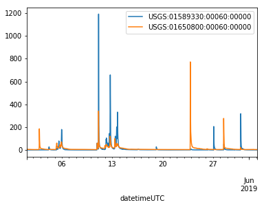
[9]:
data.df('discharge').plot()
C:\Users\Marty\Anaconda3\envs\py37hfdev\lib\site-packages\pandas\core\arrays\datetimes.py:1172: UserWarning: Converting to PeriodArray/Index representation will drop timezone information.
  "will drop timezone information.", UserWarning)
[9]:
<matplotlib.axes._subplots.AxesSubplot at 0x287dae95208>
View descriptive statistics
[10]:
data.df('discharge').describe()
[10]:
| USGS:01589330:00060:00000 | USGS:01650800:00060:00000 | |
|---|---|---|
| count | 9216.000000 | 9216.000000 |
| mean | 11.630525 | 13.615661 |
| std | 48.421805 | 29.256210 |
| min | 1.390000 | 4.850000 |
| 25% | 1.940000 | 5.530000 |
| 50% | 2.410000 | 6.610000 |
| 75% | 4.630000 | 12.800000 |
| max | 1190.000000 | 772.000000 |
Error messages
Hydrofunctions will let you know if you request something you don’t have.
[11]:
data.df('00000000')
---------------------------------------------------------------------------
ValueError                                Traceback (most recent call last)
<ipython-input-11-ba193784fd2d> in <module>
----> 1 data.df('00000000')

c:\users\marty\google drive\pydev\src\hydrofunctions\hydrofunctions\station.py in df(self, *args)
    228                     sites = self._dataframe.columns.str.contains(station_arg)
    229                     if not sites.any():
--> 230                         raise ValueError("The site '{site}' is not in this dataset.".format(site=item))
    231                 else:
    232                     raise ValueError("The argument '{item}' is not recognized.".format(item=item))

ValueError: The site '00000000' is not in this dataset.
