Comparing Three Nested Watersheds
In this notebook we’ll examine three sites along the Gwynns Falls, in Maryland. ‘Falls’ in this case is a local word for ‘River’, like in the Jones Falls or Gunpowder Falls. It doesn’t refer to a waterfall!
Because the three sites are in a row on the same river, the upstream site has a watershed that is nested inside of the middle site, which is nested inside the downstream site, which has the largest watershed.
[1]:
import hydrofunctions as hf
%matplotlib inline
The three stream gauges are:
the farthest upstream is GWYNNS FALLS NEAR DELIGHT, MD, dv01589197
the middle of stream is GWYNNS FALLS AT VILLA NOVA, MD, dv01589300
the farthest downstream is GWYNNS FALLS AT WASHINGTON BLVD AT BALTIMORE, MD, dv01589352
[2]:
streamid = ['01589197', '01589300','01589352']
# request data for our two sites for a three-year period.
sites = hf.NWIS(streamid, 'dv', start_date='2001-01-01', end_date='2003-12-31')
sites
Requested data from https://waterservices.usgs.gov/nwis/dv/?format=json%2C1.1&sites=01589197%2C01589300%2C01589352&startDT=2001-01-01&endDT=2003-12-31
[2]:
USGS:01589197: GWYNNS FALLS NEAR DELIGHT, MD
    00060: <Day>  Discharge, cubic feet per second
USGS:01589300: GWYNNS FALLS AT VILLA NOVA, MD
    00060: <Day>  Discharge, cubic feet per second
USGS:01589352: GWYNNS FALLS AT WASHINGTON BLVD AT BALTIMORE, MD
    00060: <Day>  Discharge, cubic feet per second
Start: 2001-01-01 00:00:00+00:00
End:   2003-12-31 00:00:00+00:00
[3]:
#create a dataframe of the sites
Q = sites.df('discharge')
#rename the columns
Q.columns=['Upper', 'Middle', 'Lower']
#show the first few rows of the data
Q.head()
[3]:
| Upper | Middle | Lower | |
|---|---|---|---|
| datetimeUTC | |||
| 2001-01-01 00:00:00+00:00 | 1.8 | 18.0 | 29.0 |
| 2001-01-02 00:00:00+00:00 | 1.8 | 17.0 | 28.0 |
| 2001-01-03 00:00:00+00:00 | 1.8 | 16.0 | 27.0 |
| 2001-01-04 00:00:00+00:00 | 1.8 | 17.0 | 31.0 |
| 2001-01-05 00:00:00+00:00 | 1.8 | 16.0 | 31.0 |
[4]:
#look at the descriptive statistics for each part of the stream.
#Note that the mean and standard deviation increase as you move down the stream
Q.describe()
[4]:
| Upper | Middle | Lower | |
|---|---|---|---|
| count | 1095.000000 | 1095.000000 | 1095.000000 |
| mean | 5.211306 | 44.910210 | 92.074055 |
| std | 10.177445 | 79.268103 | 173.157576 |
| min | 0.250000 | 1.860000 | 8.730000 |
| 25% | 1.590000 | 14.000000 | 27.800000 |
| 50% | 2.720000 | 24.400000 | 43.000000 |
| 75% | 5.000000 | 42.850000 | 80.800000 |
| max | 161.000000 | 1140.000000 | 2140.000000 |
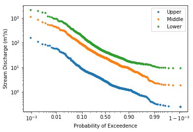
[5]:
#create a flow duration for each of the streams
hf.flow_duration(Q)
[5]:
(<Figure size 432x288 with 1 Axes>,
 <matplotlib.axes._subplots.AxesSubplot at 0x1fe91e24978>)
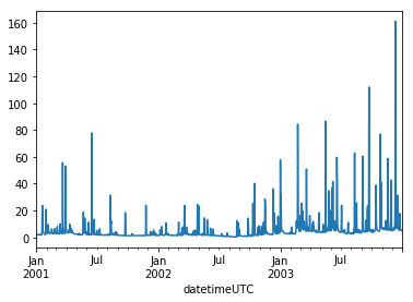
[6]:
# create a hydrograph of the upper portion of the stream.
# the .loc method selects a subset of a dataframe.
# The first item selects rows, with ':' selecting every row.
# The second item selects columns, with 'Upper' selecting the column with the 'Upper' label.
# The .plot() method plots the values in the columns on the y axis, with the rows as the x axis.
Q.loc[:, 'Upper'].plot()
C:\Users\Marty\Anaconda3\envs\py37hfdev\lib\site-packages\pandas\core\arrays\datetimes.py:1172: UserWarning: Converting to PeriodArray/Index representation will drop timezone information.
  "will drop timezone information.", UserWarning)
[6]:
<matplotlib.axes._subplots.AxesSubplot at 0x1fe920d60b8>