A Hydrofunctions Tutorial
This guide will step you through the basics of using hydrofunctions. Read more in our User’s Guide, or visit us on GitHub!
Installation
The first step before using hydrofunctions is to get it installed on your system. For scientific computing, we highly recommend using the free, open-source Anaconda distribution to load and manage all of your Python tools and packages. Once you have downloaded and installed Anaconda, or if you already have Python set up on your computer, your next step is to use the pip tool from your operating system’s command line to download hydrofunctions.
In Linux: $ pip install hydrofunctions
In Windows: C:\MyPythonWorkspace\> pip install hydrofunctions
If you have any difficulties, visit our Installation page in the User’s Guide.
Getting started in Python
From here on out, we will assume that you have installed hydrofunctions and you are working at a Python command prompt, perhaps in ipython or in a Jupyter notebook.
[1]:
# The first step is to import hydrofunctions so that we can use it here.

import hydrofunctions as hf
# This second line allows us to automatically plot diagrams in this notebook.
%matplotlib inline
Get data for a USGS streamflow gage
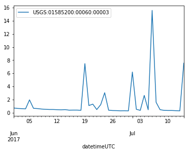
The USGS runs an amazing web service called the National Water Information System. Our first task is to download daily mean discharge data for a stream called Herring Run. Set the start date and the end date for our download, and use the site number for Herring Run (‘01585200’) to specify which stream gage we want to collect data from. Once we request the data, it will be saved to a file. If the file is already present, we’ll just use that instead of requesting it from the NWIS.
You can visit the NWIS website or use hydrocloud.org to find the site number for a stream gage near you.
[2]:
start = '2017-06-01'
end = '2017-07-14'
herring = hf.NWIS('01585200', 'dv', start, end, file='herring_july.parquet')
herring # This last command will print out a description of what we have.
Reading data from herring_july.parquet
[2]:
USGS:01585200: WEST BRANCH HERRING RUN AT IDLEWYLDE, MD
    00060: <Day>  Discharge, cubic feet per second
Start: 2017-06-01 00:00:00+00:00
End:   2017-07-14 00:00:00+00:00
Viewing our data
There are several ways to view our data. Try herring.json() or better still, use a Pandas dataframe:
[3]:
herring.df()
[3]:
| USGS:01585200:00060:00003_qualifiers | USGS:01585200:00060:00003 | |
|---|---|---|
| datetimeUTC | ||
| 2017-06-01 00:00:00+00:00 | A | 0.71 |
| 2017-06-02 00:00:00+00:00 | A | 0.64 |
| 2017-06-03 00:00:00+00:00 | A | 0.61 |
| 2017-06-04 00:00:00+00:00 | A | 0.58 |
| 2017-06-05 00:00:00+00:00 | A | 1.95 |
| 2017-06-06 00:00:00+00:00 | A | 0.66 |
| 2017-06-07 00:00:00+00:00 | A | 0.62 |
| 2017-06-08 00:00:00+00:00 | A | 0.55 |
| 2017-06-09 00:00:00+00:00 | A | 0.51 |
| 2017-06-10 00:00:00+00:00 | A | 0.48 |
| 2017-06-11 00:00:00+00:00 | A | 0.48 |
| 2017-06-12 00:00:00+00:00 | A | 0.45 |
| 2017-06-13 00:00:00+00:00 | A | 0.43 |
| 2017-06-14 00:00:00+00:00 | A | 0.46 |
| 2017-06-15 00:00:00+00:00 | A | 0.38 |
| 2017-06-16 00:00:00+00:00 | A | 0.39 |
| 2017-06-17 00:00:00+00:00 | A | 0.39 |
| 2017-06-18 00:00:00+00:00 | A | 0.36 |
| 2017-06-19 00:00:00+00:00 | A | 7.48 |
| 2017-06-20 00:00:00+00:00 | A | 1.08 |
| 2017-06-21 00:00:00+00:00 | A | 1.30 |
| 2017-06-22 00:00:00+00:00 | A | 0.47 |
| 2017-06-23 00:00:00+00:00 | A | 1.22 |
| 2017-06-24 00:00:00+00:00 | A | 3.04 |
| 2017-06-25 00:00:00+00:00 | A | 0.37 |
| 2017-06-26 00:00:00+00:00 | A | 0.32 |
| 2017-06-27 00:00:00+00:00 | A | 0.31 |
| 2017-06-28 00:00:00+00:00 | A | 0.28 |
| 2017-06-29 00:00:00+00:00 | A | 0.29 |
| 2017-06-30 00:00:00+00:00 | A | 0.27 |
| 2017-07-01 00:00:00+00:00 | A | 6.20 |
| 2017-07-02 00:00:00+00:00 | A | 0.51 |
| 2017-07-03 00:00:00+00:00 | A | 0.35 |
| 2017-07-04 00:00:00+00:00 | A | 2.63 |
| 2017-07-05 00:00:00+00:00 | A | 0.44 |
| 2017-07-06 00:00:00+00:00 | A | 15.60 |
| 2017-07-07 00:00:00+00:00 | A | 1.58 |
| 2017-07-08 00:00:00+00:00 | A | 0.45 |
| 2017-07-09 00:00:00+00:00 | A | 0.35 |
| 2017-07-10 00:00:00+00:00 | A | 0.33 |
| 2017-07-11 00:00:00+00:00 | A | 0.33 |
| 2017-07-12 00:00:00+00:00 | A | 0.30 |
| 2017-07-13 00:00:00+00:00 | A | 0.28 |
| 2017-07-14 00:00:00+00:00 | A | 7.55 |
Pandas’ dataframes give you access to hundreds of useful methods, such as .describe() and .plot():
[4]:
herring.df().describe()
[4]:
| USGS:01585200:00060:00003 | |
|---|---|
| count | 44.000000 |
| mean | 1.454091 |
| std | 2.792200 |
| min | 0.270000 |
| 25% | 0.357500 |
| 50% | 0.475000 |
| 75% | 0.802500 |
| max | 15.600000 |
[5]:
herring.df().plot()
C:\Users\Marty\Anaconda3\envs\py37hfdev\lib\site-packages\pandas\core\arrays\datetimes.py:1172: UserWarning: Converting to PeriodArray/Index representation will drop timezone information.
  "will drop timezone information.", UserWarning)
[5]:
<matplotlib.axes._subplots.AxesSubplot at 0x22f6664b198>
Multiple sites, other parameters
It’s possible to load data from several different sites at the same time, and you aren’t limited to just stream discharge.
Requests can use lists of sites:
[6]:
sites = ['380616075380701','394008077005601']
The NWIS can deliver data as daily mean values (‘dv’) or as instantaneous values (‘iv’) that can get collected as often as every five minutes!
[7]:
service = 'iv'
Depending on the site, the USGS collects groundwater levels (‘72019’), stage (‘00065’), precipitation, and more!
[8]:
pcode = '72019'
Now we’ll create a new dataset called ‘groundwater’ using the values we set up above.
Since one of the parameters gets collected every 30 minutes, and the other gets collected every 15 minutes, Hydrofunctions will interpolate values for every 15 minutes for every parameter we’ve requested. These interpolated values will be marked with a special hf.interpolate flag in the qualifiers column.
[9]:
groundwater = hf.NWIS(sites, service, '2018-01-01', '2018-01-31', parameterCd=pcode, file='groundwater.parquet')
groundwater
Reading data from groundwater.parquet
[9]:
USGS:380616075380701: SO Cf   2
    72019: <15 * Minutes>  Depth to water level, feet below land surface
USGS:394008077005601: CL Ad  47
    72019: <30 * Minutes>  Depth to water level, feet below land surface
Start: 2018-01-01 05:00:00+00:00
End:   2018-02-01 04:45:00+00:00
Calculate the mean for every data column:
[10]:
groundwater.df().mean()
[10]:
USGS:380616075380701:72019:00000    1.215141
USGS:394008077005601:72019:00000    3.206111
dtype: float64
View the data in a specially styled graph!
[11]:
groundwater.df().plot(marker='o', mfc='white', ms=4, mec='black', color='black')
[11]:
<matplotlib.axes._subplots.AxesSubplot at 0x22f667facc0>
Learning more
hydrofunctions comes with a variety of built-in help functions that you can access from the command line, in addition to our online User’s Guide.
Jupyter Notebooks provide additional helpful shortcuts, such as code completion. This will list all of the available methods for an object just by hitting like this: herring.<TAB> this is equivalent to using dir(herring) to list all of the methods available to you.
Typing help() or dir() for different objects allows you to access additional information. help(hf.NWIS) is equivalent to just using a question mark like this: ?hf.NWIS
[12]:
help(hf.NWIS)
Help on class NWIS in module hydrofunctions.station:

class NWIS(Station)
 |  NWIS(site=None, service='dv', start_date=None, end_date=None, stateCd=None, countyCd=None, bBox=None, parameterCd='all', period=None, file=None)
 |
 |  A class for working with data from the USGS NWIS service.
 |
 |  description
 |
 |  Args:
 |      site (str or list of strings):
 |          a valid site is '01585200' or ['01585200', '01646502']. Default is
 |          None. If site is not specified, you will need to select sites using
 |          stateCd or countyCd.
 |
 |      service (str):
 |          can either be 'iv' or 'dv' for instantaneous or daily data.
 |          'dv'(default): daily values. Mean value for an entire day.
 |          'iv': instantaneous value measured at this time. Also known
 |          as 'Real-time data'. Can be measured as often as every
 |          five minutes by the USGS. 15 minutes is more typical.
 |
 |      start_date (str):
 |         should take on the form 'yyyy-mm-dd'
 |
 |      end_date (str):
 |          should take on the form 'yyyy-mm-dd'
 |
 |      stateCd (str):
 |          a valid two-letter state postal abbreviation, such as 'MD'. Default
 |          is None. Selects all stations in this state. Because this type of
 |          site selection returns a large number of sites, you should limit
 |          the amount of data requested for each site.
 |
 |      countyCd (str or list of strings):
 |          a valid county FIPS code. Default is None. Requests all stations
 |          within the county or list of counties. See https://en.wikipedia.org/wiki/FIPS_county_code
 |          for an explanation of FIPS codes.
 |
 |      bBox (str, list, or tuple):
 |          a set of coordinates that defines a bounding box.
 |              * Coordinates are in decimal degrees.
 |              * Longitude values are negative (west of the prime meridian).
 |              * Latitude values are positive (north of the equator).
 |              * comma-delimited, no spaces, if provided as a string.
 |              * The order of the boundaries should be: "West,South,East,North"
 |              * Example: "-83.000000,36.500000,-81.000000,38.500000"
 |
 |      parameterCd (str or list of strings):
 |          NWIS parameter code. Usually a five digit code. Default is 'all'.
 |          A valid code can also be given as a list: parameterCd=['00060','00065']
 |          This will request data for this parameter.
 |
 |              * if value is 'all', or no value is submitted, then NWIS will                 return every parameter collected at this site. (default option)
 |              * stage: '00065'
 |              * discharge: '00060'
 |              * not all sites collect all parameters!
 |              * See https://nwis.waterdata.usgs.gov/usa/nwis/pmcodes for full list
 |
 |      period (str):
 |          NWIS period code. Default is None.
 |              * Format is "PxxD", where xx is the number of days before                 today, with a maximum of 999 days accepted.
 |              * Either use start_date or period, but not both.
 |
 |  Method resolution order:
 |      NWIS
 |      Station
 |      builtins.object
 |
 |  Methods defined here:
 |
 |  __init__(self, site=None, service='dv', start_date=None, end_date=None, stateCd=None, countyCd=None, bBox=None, parameterCd='all', period=None, file=None)
 |      Initialize self.  See help(type(self)) for accurate signature.
 |
 |  __repr__(self)
 |      Return repr(self).
 |
 |  df(self, *args)
 |      Return a subset of columns from the dataframe.
 |
 |      Args:
 |          '': If no args are provided, the entire dataframe will be returned.
 |
 |          str 'all': the entire dataframe will be returned.
 |
 |          str 'data': all of the parameters will be returned, with no flags.
 |
 |          str 'flags': Only the _qualifier flags will be returned. Unless the             flags arg is provided, only data columns will be returned. Visit             https://waterdata.usgs.gov/usa/nwis/uv?codes_help#dv_cd1 to see a             more complete listing of possible codes.
 |
 |          str 'discharge' or 'q': discharge columns ('00060') will be returned.
 |
 |          str 'stage': Gauge height columns ('00065') will be returned.
 |
 |          int any five digit number: any matching parameter columns will be returned. '00065' returns stage, for example.
 |
 |          int any eight to twelve digit number: any matching stations will be returned.
 |
 |  get_data(self)
 |
 |  read(self, file)
 |
 |  save(self, file)
 |
 |  ----------------------------------------------------------------------
 |  Data descriptors inherited from Station:
 |
 |  __dict__
 |      dictionary for instance variables (if defined)
 |
 |  __weakref__
 |      list of weak references to the object (if defined)
 |
 |  ----------------------------------------------------------------------
 |  Data and other attributes inherited from Station:
 |
 |  station_dict = {}
Advanced techniques
Download data for a large number of sites
[13]:
sites = ['07227500', '07228000', '07235000', '07295500', '07297910', '07298500', '07299540',
         '07299670', '07299890', '07300000', '07301300', '07301410', '07308200', '07308500', '07311600',
         '07311630', '07311700', '07311782', '07311783', '07311800', '07311900', '07312100', '07312200',
         '07312500', '07312700', '07314500', '07314900', '07315200', '07315500', '07342465', '07342480',
         '07342500', '07343000', '07343200', '07343500', '07344210', '07344500', '07346000']
mult = hf.NWIS(sites, "dv", "2018-01-01", "2018-01-31", file='mult.parquet')
print('No. sites: {}'.format(len(sites)))
Reading data from mult.parquet
No. sites: 38
This will calculate the mean value for each site.
[14]:
mult.df().mean()
[14]:
USGS:07227500:00010:00001       6.848387
USGS:07227500:00010:00002       0.661290
USGS:07227500:00010:00003       3.254839
USGS:07227500:00060:00003      51.880645
USGS:07227500:00065:00003       1.233710
USGS:07227500:00095:00001    5968.333333
USGS:07227500:00095:00002    5648.571429
USGS:07227500:00095:00003    5788.333333
USGS:07228000:00060:00003      57.938710
USGS:07228000:00065:00003       1.429032
USGS:07235000:00060:00001       0.657742
USGS:07235000:00060:00002       0.462581
USGS:07235000:00060:00003       0.558065
USGS:07235000:00065:00003       4.381613
USGS:07295500:00060:00001       0.000000
USGS:07295500:00060:00002       0.000000
USGS:07295500:00060:00003       0.000000
USGS:07295500:00065:00001       0.606452
USGS:07295500:00065:00002       0.600000
USGS:07295500:00065:00003       0.600000
USGS:07297910:00060:00001      24.383871
USGS:07297910:00060:00002      14.901290
USGS:07297910:00060:00003      19.103226
USGS:07297910:00065:00001       6.003148
USGS:07297910:00065:00002       5.941111
USGS:07297910:00065:00003       5.967778
USGS:07298500:00060:00001      10.042581
USGS:07298500:00060:00002       7.213548
USGS:07298500:00060:00003       8.730968
USGS:07298500:00065:00001       4.830000
                                ...
USGS:07342500:00065:00002       2.810645
USGS:07342500:00065:00003       2.835161
USGS:07343000:00060:00001      68.566452
USGS:07343000:00060:00002      14.491935
USGS:07343000:00060:00003      36.442258
USGS:07343000:00065:00001       1.601935
USGS:07343000:00065:00002       1.318065
USGS:07343000:00065:00003       1.468065
USGS:07343200:00060:00003      76.200000
USGS:07343500:00060:00001      52.474194
USGS:07343500:00060:00002      34.600000
USGS:07343500:00060:00003      43.445161
USGS:07343500:00065:00001       2.986452
USGS:07343500:00065:00002       2.609839
USGS:07343500:00065:00003       2.794032
USGS:07344210:00060:00001    1304.306452
USGS:07344210:00060:00002    1208.258065
USGS:07344210:00065:00001      13.347419
USGS:07344210:00065:00002      12.885161
USGS:07344210:00065:00003      13.119032
USGS:07344500:00060:00001      10.138065
USGS:07344500:00060:00002       6.139677
USGS:07344500:00060:00003       7.929032
USGS:07344500:00065:00001       5.570323
USGS:07344500:00065:00002       5.401613
USGS:07344500:00065:00003       5.482258
USGS:07346000:00060:00001     287.387097
USGS:07346000:00060:00002     283.548387
USGS:07346000:00060:00003     285.387097
USGS:07346000:00065:00003       8.185806
Length: 164, dtype: float64
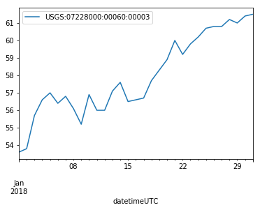
Plot just the discharge data for one site in the list:
[15]:
mult.df('07228000', 'discharge').plot()
[15]:
<matplotlib.axes._subplots.AxesSubplot at 0x22f66758780>
List some of the data available to you in a dataframe.
[16]:
mult
[16]:
USGS:07227500: Canadian Rv nr Amarillo, TX
    00010: <Day>  Temperature, water, degrees Celsius
    00060: <Day>  Discharge, cubic feet per second
    00065: <Day>  Gage height, feet
    00095: <Day>  Specific conductance, water, unfiltered, microsiemens per centimeter at 25 degrees Celsius
USGS:07228000: Canadian Rv nr Canadian, TX
    00060: <Day>  Discharge, cubic feet per second
    00065: <Day>  Gage height, feet
USGS:07235000: Wolf Ck at Lipscomb, TX
    00060: <Day>  Discharge, cubic feet per second
    00065: <Day>  Gage height, feet
USGS:07295500: Tierra Blanca Ck abv Buffalo Lk nr Umbarger, TX
    00060: <Day>  Discharge, cubic feet per second
    00065: <Day>  Gage height, feet
USGS:07297910: Pr Dog Twn Fk Red Rv nr Wayside, TX
    00060: <Day>  Discharge, cubic feet per second
    00065: <Day>  Gage height, feet
USGS:07298500: Pr Dog Twn Fk Red Rv nr Brice, TX
    00060: <Day>  Discharge, cubic feet per second
    00065: <Day>  Gage height, feet
USGS:07299540: Pr Dog Twn Fk Red Rv nr Childress, TX
    00060: <Day>  Discharge, cubic feet per second
    00065: <Day>  Gage height, feet
USGS:07299670: Groesbeck Ck at SH 6 nr Quanah, TX
    00060: <Day>  Discharge, cubic feet per second
    00065: <Day>  Gage height, feet
USGS:07299890: Lelia Lk Ck bl Bell Ck nr Hedley, TX
    00060: <Day>  Discharge, cubic feet per second
    00065: <Day>  Gage height, feet
USGS:07300000: Salt Fk Red Rv nr Wellington, TX
    00060: <Day>  Discharge, cubic feet per second
    00065: <Day>  Gage height, feet
USGS:07301300: N Fk Red Rv nr Shamrock, TX
    00060: <Day>  Discharge, cubic feet per second
USGS:07301410: Sweetwater Ck nr Kelton, TX
    00060: <Day>  Discharge, cubic feet per second
USGS:07308200: Pease Rv nr Vernon, TX
    00060: <Day>  Discharge, cubic feet per second
    00065: <Day>  Gage height, feet
USGS:07308500: Red Rv nr Burkburnett, TX
    00060: <Day>  Discharge, cubic feet per second
    00065: <Day>  Gage height, feet
USGS:07311700: N Wichita Rv nr Truscott, TX
    00060: <Day>  Discharge, cubic feet per second
    00065: <Day>  Gage height, feet
USGS:07311800: S Wichita Rv nr Benjamin, TX
    00010: <Day>  Temperature, water, degrees Celsius
    00060: <Day>  Discharge, cubic feet per second
    00065: <Day>  Gage height, feet
    00095: <Day>  Specific conductance, water, unfiltered, microsiemens per centimeter at 25 degrees Celsius
USGS:07311900: Wichita Rv nr Seymour, TX
    00060: <Day>  Discharge, cubic feet per second
    00065: <Day>  Gage height, feet
USGS:07312100: Wichita Rv nr Mabelle, TX
    00060: <Day>  Discharge, cubic feet per second
    00065: <Day>  Gage height, feet
USGS:07312200: Beaver Ck nr Electra, TX
    00060: <Day>  Discharge, cubic feet per second
    00065: <2 * Days>  Gage height, feet
USGS:07312500: Wichita Rv at Wichita Falls, TX
    00010: <Day>  Temperature, water, degrees Celsius
    00060: <Day>  Discharge, cubic feet per second
    00065: <Day>  Gage height, feet
    00095: <Day>  Specific conductance, water, unfiltered, microsiemens per centimeter at 25 degrees Celsius
USGS:07312700: Wichita Rv nr Charlie, TX
    00010: <Day>  Temperature, water, degrees Celsius
    00060: <Day>  Discharge, cubic feet per second
    00065: <Day>  Gage height, feet
    00095: <Day>  Specific conductance, water, unfiltered, microsiemens per centimeter at 25 degrees Celsius
USGS:07314500: Little Wichita Rv nr Archer City, TX
    00060: <Day>  Discharge, cubic feet per second
    00065: <Day>  Gage height, feet
USGS:07314900: Little Wichita Rv abv Henrietta, TX
    00060: <Day>  Discharge, cubic feet per second
    00065: <Day>  Gage height, feet
USGS:07315200: E Fk Little Wichita Rv nr Henrietta, TX
    00060: <Day>  Discharge, cubic feet per second
    00065: <Day>  Gage height, feet
USGS:07315500: Red Rv nr Terral, OK
    00060: <Day>  Discharge, cubic feet per second
    00065: <Day>  Gage height, feet
USGS:07342465: S Sulphur Rv at Commerce, TX
    00060: <Day>  Discharge, cubic feet per second
    00065: <Day>  Gage height, feet
USGS:07342480: Middle Sulphur Rv at Commerce, TX
    00060: <Day>  Discharge, cubic feet per second
    00065: <Day>  Gage height, feet
USGS:07342500: S Sulphur Rv nr Cooper, TX
    00060: <Day>  Discharge, cubic feet per second
    00065: <Day>  Gage height, feet
USGS:07343000: N Sulphur Rv nr Cooper, TX
    00060: <Day>  Discharge, cubic feet per second
    00065: <Day>  Gage height, feet
USGS:07343200: Sulphur Rv nr Talco, TX
    00060: <Day>  Discharge, cubic feet per second
USGS:07343500: White Oak Ck nr Talco, TX
    00060: <Day>  Discharge, cubic feet per second
    00065: <Day>  Gage height, feet
USGS:07344210: Sulphur Rv nr Texarkana, TX
    00060: <Day>  Discharge, cubic feet per second
    00065: <Day>  Gage height, feet
USGS:07344500: Big Cypress Ck nr Pittsburg, TX
    00060: <Day>  Discharge, cubic feet per second
    00065: <Day>  Gage height, feet
USGS:07346000: Big Cypress Bayou nr Jefferson, TX
    00060: <Day>  Discharge, cubic feet per second
    00065: <Day>  Gage height, feet
Start: 2018-01-01 00:00:00+00:00
End:   2018-01-31 00:00:00+00:00
Create a table of discharge data
.head() only show the first five.tail() only show the last five[17]:
mult.df('discharge').head()
[17]:
| USGS:07227500:00060:00003 | USGS:07228000:00060:00003 | USGS:07235000:00060:00001 | USGS:07235000:00060:00002 | USGS:07235000:00060:00003 | USGS:07295500:00060:00001 | USGS:07295500:00060:00002 | USGS:07295500:00060:00003 | USGS:07297910:00060:00001 | USGS:07297910:00060:00002 | ... | USGS:07343500:00060:00002 | USGS:07343500:00060:00003 | USGS:07344210:00060:00001 | USGS:07344210:00060:00002 | USGS:07344500:00060:00001 | USGS:07344500:00060:00002 | USGS:07344500:00060:00003 | USGS:07346000:00060:00001 | USGS:07346000:00060:00002 | USGS:07346000:00060:00003 | |
|---|---|---|---|---|---|---|---|---|---|---|---|---|---|---|---|---|---|---|---|---|---|
| datetimeUTC | |||||||||||||||||||||
| 2018-01-01 00:00:00+00:00 | 43.0 | 53.6 | 0.55 | 0.40 | 0.46 | 0.0 | 0.0 | 0.0 | 30.9 | 25.9 | ... | 35.8 | 37.7 | 774.0 | 756.0 | 4.82 | 4.00 | 4.44 | 285.0 | 283.0 | 284.0 |
| 2018-01-02 00:00:00+00:00 | 52.9 | 53.8 | 0.61 | 0.36 | 0.48 | 0.0 | 0.0 | 0.0 | 35.9 | 30.9 | ... | 32.5 | 34.0 | 1360.0 | 763.0 | 5.27 | 3.70 | 4.32 | 285.0 | 284.0 | 285.0 |
| 2018-01-03 00:00:00+00:00 | 51.7 | 55.7 | 0.55 | 0.46 | 0.51 | 0.0 | 0.0 | 0.0 | 43.3 | 18.8 | ... | 30.4 | 31.6 | 1510.0 | 1360.0 | 6.10 | 4.97 | 5.29 | 285.0 | 284.0 | 284.0 |
| 2018-01-04 00:00:00+00:00 | 50.7 | 56.6 | 0.51 | 0.46 | 0.48 | 0.0 | 0.0 | 0.0 | 30.9 | 14.7 | ... | 27.1 | 28.8 | 1530.0 | 1510.0 | 7.17 | 6.10 | 6.66 | 284.0 | 283.0 | 283.0 |
| 2018-01-05 00:00:00+00:00 | 53.8 | 57.0 | 0.51 | 0.46 | 0.49 | 0.0 | 0.0 | 0.0 | 30.9 | 16.0 | ... | 23.6 | 25.5 | 1530.0 | 1520.0 | 7.39 | 6.61 | 7.02 | 284.0 | 282.0 | 283.0 |
5 rows × 73 columns
Download all streamflow data for the state of Virginia
[18]:
# Use this carefully! You can easily request more data than you will know what to do with.
start = "2017-01-01"
end = "2017-12-31"
param = '00060'
virginia = hf.NWIS(None, "dv", start, end, parameterCd=param, stateCd='va', file='virginia.parquet')
Reading data from virginia.parquet
[19]:
# Calculate the mean for each site.
virginia.df('discharge').mean()
[19]:
USGS:01613900:00060:00003      12.901726
USGS:01615000:00060:00003      41.219260
USGS:01616100:00060:00003       8.948493
USGS:01620500:00060:00003      17.857973
USGS:01621050:00060:00003       3.844548
USGS:01622000:00060:00003     277.692055
USGS:01625000:00060:00003     245.340548
USGS:01626000:00060:00003     106.207123
USGS:01626850:00060:00003     143.700000
USGS:01627500:00060:00003     184.487397
USGS:01628500:00060:00003     748.202740
USGS:01629500:00060:00003     990.643836
USGS:01631000:00060:00003    1114.293151
USGS:01632000:00060:00003     124.048740
USGS:01632082:00060:00003      17.520329
USGS:01632900:00060:00003      39.136493
USGS:01633000:00060:00003     218.096712
USGS:01634000:00060:00003     361.363562
USGS:01634500:00060:00003      77.218795
USGS:01635500:00060:00003      48.196192
USGS:01636316:00060:00003      16.360575
USGS:01636690:00060:00003      11.838795
USGS:01638350:00060:00003      25.122712
USGS:01638420:00060:00003      19.026932
USGS:01638480:00060:00003      66.770411
USGS:01643590:00060:00003       5.074493
USGS:01643700:00060:00003      98.993425
USGS:01643805:00060:00003      31.099041
USGS:01643880:00060:00003      42.124575
USGS:01644000:00060:00003     271.511233
                                ...
USGS:02076000:00060:00003    2715.035616
USGS:02077000:00060:00003     495.344384
USGS:02079640:00060:00003      30.671205
USGS:03164000:00060:00003    1809.479452
USGS:03165000:00060:00003      69.004110
USGS:03165500:00060:00003    2113.663014
USGS:03167000:00060:00003     268.287671
USGS:03168000:00060:00003    3159.178082
USGS:03170000:00060:00003     366.520548
USGS:03171000:00060:00003    3966.383562
USGS:03173000:00060:00003     335.324932
USGS:03175500:00060:00003     321.495616
USGS:03176500:00060:00003    5021.671233
USGS:03177710:00060:00003      62.864110
USGS:03207800:00060:00003     385.552877
USGS:03208500:00060:00003     330.526575
USGS:03208950:00060:00003      85.020000
USGS:03209000:00060:00003     294.153973
USGS:03471500:00060:00003     109.356712
USGS:03473000:00060:00003     501.227123
USGS:03474000:00060:00003     171.507123
USGS:03475000:00060:00003     254.800822
USGS:03478400:00060:00003      34.246301
USGS:03488000:00060:00003     296.555890
USGS:03490000:00060:00003     923.371507
USGS:03524000:00060:00003     700.853151
USGS:03524500:00060:00003     143.473973
USGS:03527000:00060:00003    1510.515068
USGS:03529500:00060:00003     187.819178
USGS:03531500:00060:00003     554.865479
Length: 190, dtype: float64
Plot all streamflow data for the state of Virginia
[20]:
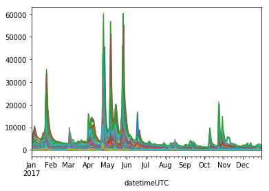
# There are so many sites that we can't read them all!
virginia.df('q').plot(legend=None)
[20]:
<matplotlib.axes._subplots.AxesSubplot at 0x22f67bb6588>
Download all streamflow data for Fairfax and Prince William counties in the state of Virginia
[21]:
start = "2017-01-01"
end = "2017-12-31"
county = hf.NWIS(None, "dv", start, end, parameterCd='00060', countyCd=['51059', '51061'], file='PG.parquet')
Reading data from PG.parquet
[22]:
county.df('data').head()
[22]:
| USGS:01645704:00060:00003 | USGS:01645762:00060:00003 | USGS:01646000:00060:00003 | USGS:01646305:00060:00003 | USGS:01654000:00060:00003 | USGS:01654500:00060:00003 | USGS:01655794:00060:00003 | USGS:01656000:00060:00003 | USGS:01656903:00060:00003 | USGS:01661977:00060:00003 | USGS:01664000:00060:00003 | |
|---|---|---|---|---|---|---|---|---|---|---|---|
| datetimeUTC | |||||||||||
| 2017-01-01 00:00:00+00:00 | 1.89 | 0.92 | 19.0 | 0.40 | 3.88 | 0.49 | NaN | 9.55 | 1.12 | NaN | 205.0 |
| 2017-01-02 00:00:00+00:00 | 4.69 | 1.44 | 28.8 | 2.17 | 18.30 | 2.02 | NaN | 9.70 | 2.18 | NaN | 200.0 |
| 2017-01-03 00:00:00+00:00 | 33.60 | 9.79 | 298.0 | 20.10 | 225.00 | 23.10 | NaN | 128.00 | 23.50 | NaN | 256.0 |
| 2017-01-04 00:00:00+00:00 | 13.40 | 2.87 | 95.6 | 1.26 | 24.10 | 2.17 | NaN | 90.50 | 7.46 | NaN | 761.0 |
| 2017-01-05 00:00:00+00:00 | 6.06 | 1.74 | 41.4 | 0.73 | 9.77 | 1.14 | NaN | 36.50 | 3.20 | NaN | 650.0 |
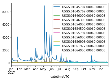
Plot all streamflow data for Fairfax and Prince William counties in the state of Virginia
[23]:
county.df('data').plot()
[23]:
<matplotlib.axes._subplots.AxesSubplot at 0x22f67bd87b8>
Thanks for using hydrofunctions!
We would love to hear your comments and suggestions!
